Examples of how commonly reported construction data can often be misused – Construction Spending and Construction Starts

Construction Grew $41 billion, 3.3%, from 2017 to 2018

An increase in construction spending is often referred to as growth for the industry, but that is incorrect. Construction spending measures the change in the dollar value of work performed, not the volume of work performed.

The difference between spending (or revenue) and volume can be explained by a simple example, the Crate of Apples. A farm stand sold a crate of apples last year for $100. Costs have gone up. Today the same size crate of apples sells for $110. Farm stand revenues increased 10%, but the amount of business volume did not increase. Volume of sales is still one crate of apples. All the increase in revenue was inflation.

The $41 billion increase in construction spending from $1.266 trillion in 2017 to $1.307 trillion in 2018 is a 3.3% increase. However, construction inflation for that period averaged 4.7%. Construction inflation adds only cost, not volume, to the amount of work. Construction spending is measured in current dollars, actual dollars spent within the year in the value that year. Construction volume is measured in constant dollars, adjusted for inflation, so any and all years can be compared to each other.

Real construction volume adjusted for inflation actually decreased 1.4% from 2017 to 2018.

Total Construction volume, after accounting for inflation, has been down for five of the last six quarters. Construction volume peaked from Q1 2017 to Q1 2018, is now down 6% from the 2018 peak.

Construction volume is not directly reported. It is not a commonly referenced industry measure reported in the news. But it is a more important indicator of activity in the industry than spending. Volume is found only through analysis of spending and inflation data.

Another common misrepresentation using spending data relates to jobs growth. Jobs growth is often compared to spending growth where a 3% to 4% increase in jobs from year to year is substantiated if we have a similar 3% to 4% growth in spending. However, current $ spending is not yet adjusted for inflation and does not represent growth in real volume of work. Jobs must be compared to volume. Real volume increases are represented by constant $, or construction spending adjusted for inflation.

In the last 2 years jobs have increased by about 8% but real construction volume has decreased by about 6%. In recent years, construction volume has not supported jobs growth.

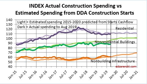
Construction Starts Predict Changes in Spending

Two very important criteria must be known about new construction starts in order to properly predict spending.

1st – To predict spending from new starts, the starts data must be spread over time using an appropriate cash flow curve. A simple illustrative spending pattern for nonresidential buildings starts, or a typical cash flow curve, for total starts within a year is: 20% of the revenue gets spent in the 1st year, 50% in the 2nd year and 30% in the 3rd year. This shows predicting spending in any given year is dependent on several previous years of starts.

Multi-billion $ highway projects, manufacturing facilities, power projects and transportation terminals often have much longer duration cash flow curves. In other words, if your intent is to predict construction spending in 2019, you need to know what starts were at a minimum in 2017 and 2018, and in many cases back to 2016 or even 2015.

Starts spread over time with cash flow curves predict spending.

2nd – For new construction starts survey sample to be used to compare to itself from year to year to predict growth in spending, sample size must be known. Starts data captures a share of the total market or a portion of all construction, on average about 60% of all construction. The easiest way to see this is compare total construction starts to total spending. Starts from 2016 to 2019 range from $750 billion to $800 billion while spending in those years ranges from $1,200 billion to $1,300 billion. From this we see starts capture a share of the total market. Any time a survey of a total population is used to forecast the total, the survey share of total must be considered.  If sample size is not constant, the apparent growth in starts does not all reflect real growth in spending.

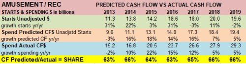
Amusement/Recreation is an example that shows starts that generate a predicted cash flow pretty well balanced with actual spending from year to year. The share of starts in the survey is fairly consistent never varying from 63% to 66% from year to year.

Office provides an example of variation in sample share of total. Starts generate predicted cash flow that increased substantially from 49% to 57% and remained higher compared to actual spending.

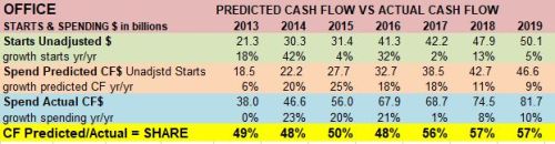
Office starts increased from $21 billion in 2013 to $50 billion in 2019. This data generates the predicted cash flow that is compared to actual spending. To predict total spending from unadjusted starts, unadjusted starts CF$ are factored up (divided by) share of total market. If the share of market captured in the survey remained constant then the predicted spending would remain close to 50%. 

CF$ Predicted/Actual shows that Cash Flow Share of actual spending was 48%-50% for several years but then jumped to 56%-57%. The predicted cash flow generated from the increase in starts is not entirely representative of an increase in spending but represents the combined value of the expected increase in spending and an increase in share of market data captured.

Starts cash flow and starts survey share of total spending are never directly known or published. These factors are found only through analysis of the data.

The Educational market data shows a similar situation as Office data. Starts generate predicted cash flow that increased substantially compared to actual spending.

Starts data generate predicted cash flow to forecast spending. This requires tracking share of total market captured in the starts survey data to account for any growth in the market share captured vs growth in predicted spending.